 -
Spectral Contamination and Alignment Rupture in Transformer Geometry
Micro-summary — details in the book
Abstract
As open-source large language models (LLMs) rapidly proliferate, the threat of data contamination—where training corpora inadvertently include benchmark test sets, alignment datasets, or web-scraped copyrighted material—has escalated into a critical concern for both safety and scientific validity. Contaminated models often exhibit deceptively high performance while relying on latent memorization, thereby undermining generalization, alignment, and trust. Existing metrics, such as token-level leakage indices, depend on explicit overlaps with held-out evaluation sets. However, such approaches are limited in scope and blind to subtle forms of semantic leakage that may evade surface-level matching.
We introduce SCAR (Spectral Contamination and Alignment Rupture), a novel diagnostic framework that identifies and quantifies contamination through the lens of latent geometry and epistemic dynamics. SCAR analyzes three complementary signals across transformer layers—spectral curvature, thermodynamic length, and belief vector field drift—to construct a unified representation of model behavior, known as the neural DNA (nDNA) trajectory. Clean models exhibit smooth, stable nDNA trajectories reflecting robust reasoning effort and internal consistency, while contaminated models manifest sharp geometric ruptures and shortcut patterns, even when outputs appear fluent and aligned.
To operationalize this framework, we propose the SCAR Score, a quantitative indicator of alignment rupture grounded in latent distortions rather than token overlap. We curate SCAR-Bench, a benchmark suite of pretraining and fine-tuning contamination scenarios across LLaMA and Mistral families, including adversarial leaks, benchmark injections, and alignment-simulation artifacts. Our experiments show that SCAR reliably detects contamination signatures that remain invisible to conventional metrics.
The SCAR framework draws deep conceptual motivation from biological systems, where genomic integrity and regulatory balance are crucial for healthy function. Just as the overexpression of a single gene can lead to cancer or autoimmune disorders, contamination in LLMs causes the overactivation of memorized latent pathways, bypassing robust reasoning. The model does not “understand”—it simply remembers too well. This shortcutting behavior resembles oncogenic triggers: minor local shifts in regulatory structure produce cascading effects on system-wide behavior. By treating layerwise activations as a form of neural genomics, SCAR enables the detection of such epistemic mutations, offering a path toward more trustworthy and biologically inspired interpretability in AI.
Inspiration
The Epistemic Wound: Why We Need SCAR
Large language models increasingly achieve striking benchmark scores, yet growing evidence shows these gains can coexist with contamination, shortcut learning, and brittle alignment—an epistemic wound that affects how a model arrives at an answer rather than what it outputs [1, 2, 3, 4]. Output-level checks (e.g., lexical overlap or reference similarity) often miss this wound because paraphrases, templatic variants, or preference-style leakage can mask direct reuse [5, 6]. To diagnose the wound, we must examine the model’s internal trajectory—its layerwise geometry and effort allocation—using tools that are sensitive to representational change and pathway distortions [7, 8, 9]. SCAR advances this structural view: it operationalizes contamination and alignment rupture as detectable discontinuities in a model’s neural DNA (nDNA), coupling spectral curvature, thermodynamic effort, and belief-vector drift into a paraphrase-robust, layer-localizing diagnostic and a calibrated score for auditing open-source models at scale.
Open-Source Acceleration, New Contamination Channels
Open-source LLMs (e.g., LLaMA-, Mistral-, Gemma-family derivatives) have unlocked rapid iteration—but also new data-supply-chain risks [1, 2]. In practice, “contamination” is not limited to verbatim benchmark leakage. It now includes: [3, 10]
- Benchmark seepage: exact items, near-paraphrases, templated variants, translations, or answer keys entering pretraining/fine-tuning [11, 12, 13, 14].
- Preference seepage: alignment datasets (e.g., helpful/harmless dialogs, safety exemplars) internalized as patterns of imitation rather than principles of preference [15, 16, 17, 18, 19].
- Derivative echo: self-distillation and instruction-tuning pipelines that recycle model outputs which already encode hidden test items or alignment style [20, 18, 19].
- Feedback loops: synthetic augmentation that repeatedly samples from contaminated distributions, amplifying shortcuts [21].
Crucially, contamination is not the same as “knowing the subject.” It is exposure during training to evaluation artifacts or alignment exemplars in a form that enables shortcut solutions at test time. Such shortcuts inflate headline scores while degrading epistemic integrity, external validity, and safety [2, 10].
Shortcut Learning Has a Shape
Models that overfit to leaked artifacts often produce correct outputs for the wrong reasons. Instead of composing evidence or reasoning, they retrieve shallow traces or style cues. We argue these failures are not merely lexical; they possess geometric signatures in the model’s internal trajectory [4, 22, 23, 24, 5]. Let \(\kappa_\ell\) denote spectral curvature of layer \(\ell\) (a shape descriptor of local representational change), \(\mathcal{L}_\ell\) the incremental thermodynamic effort (path length under a chosen metric), and \(\|\mathbf{v}_\ell\|\) the belief-vector drift (steering magnitude toward the produced answer under gradients). Then:
Clean regimes exhibit smooth, slowly varying nDNA with moderate curvature, consistent effort allocation across layers, and stable, task-conditioned belief drift.
Contaminated regimes exhibit ruptures: sharp \(\kappa_\ell\) spikes (kinks), abnormal dips or bursts in \(\mathcal{L}_\ell\) (effort misallocation), and abrupt changes in \(\|\mathbf{v}_\ell\|\) aligning with lexical/projector subspaces.
Intuitively, when a model switches from reasoning to recall, its path bends suddenly toward a memorized basin—shortening effort along intermediate steps while increasing curvature at a narrow band of late layers. This is the epistemic wound we seek to detect [7, 8, 9].
Why Surface Detectors Fail
Most existing checks—n-gram overlap, cosine similarity to references, instruction-style similarity—are brittle under paraphrase, translation, template remixes, and preference leakage (where only style leaks). They test the output but not the process. By contrast, structural diagnostics ask: Did the model follow a stable epistemic path, or did it collapse into a shortcut manifold? This shift—from lexical matching to path geometry—is essential for paraphrase-robust auditing [5, 6, 25].
Threat Model, Scope, and Confounders
We focus on contamination that induces repeatable latent shortcuts across prompts from the same task family. We explicitly consider and control for benign confounders:
- Compute/implementation effects: quantization, activation checkpointing, KV-caching—can perturb \(\mathcal{L}_\ell\). Control via fixed inference settings and sensitivity bands [26].
- Prompt format/length: formatting alone can shift trajectories. Control via multi-format evaluation and reporting prompt ensembles [25, 27].
- Domain adaptation vs. contamination: genuine adaptation can reshape nDNA smoothly; contamination induces localized kinks. Distinguish by smoothness tests and anchor-relative deltas (see below) [7, 8].
Anchor protocol. Wherever possible, we compare a suspect model against a clean anchor from the same family/size. We analyze \(\Delta\kappa_\ell\), \(\Delta\mathcal{L}_\ell\), and \(\Delta\|\mathbf{v}_\ell\|\) to reduce family- and scale-specific bias [8].
Design Principles for Structural Diagnostics
P1 — Paraphrase robustness. Signals must remain discriminative under paraphrase/translation of prompts and answers [5, 6].
P2 — Layerwise localization. Diagnostics should localize rupture layers (late-stage kinks) rather than only produce a global scalar [7, 9].
P3 — Family comparability. Normalization and anchor-relative deltas should enable comparisons across model families and sizes [8].
P4 — Falsifiability. Predictions must be testable under controlled injections and removals of leaked items [3, 10].
Operationalizing the Epistemic Wound with SCAR
SCAR treats contamination as a structural pathology. It couples (i) per-layer geometry (\(\kappa_\ell\)), (ii) path effort (\(\mathcal{L}_\ell\)), and (iii) epistemic steering (\(\|\mathbf{v}_\ell\|\)) with:
- Rupture detection: identify contiguous bands where \(\kappa_\ell\) exceeds calibrated percentiles while \(\mathcal{L}_\ell\) simultaneously deviates from anchor bands; confirm with a drift realignment test on \(\|\mathbf{v}_\ell\|\) [7, 8].
- nDNA visualization: show the full layerwise trajectory for qualitative auditing and case study analysis [9].
- SCAR score: a calibrated, z-scored combination of \(\{\kappa_\ell, \mathcal{L}_\ell, \|\mathbf{v}_\ell\|\}\) with FDR-controlled layer aggregation to produce a robust scalar for triage [3].
Testable Predictions (Pre-Registered)
P1 Localized kinks: Controlled injection of benchmark items into fine-tuning will induce late-layer \(\kappa_\ell\) spikes with concurrent \(\mathcal{L}_\ell\) dips in the same band [3].
P2 Paraphrase resilience: Under paraphrase/translation of contaminated items, surface overlap metrics degrade, but SCAR rupture bands remain stable [5].
P3 Anchor separation: For a clean anchor vs. contaminated sibling, \(\Delta\kappa_\ell\) and \(\Delta\mathcal{L}_\ell\) separate with AUC > 0.8 at fixed FPR [8].
P4 Benign controls: Changing only prompt formatting or sequence length perturbs signals smoothly (no narrow rupture bands) [25, 27].
What SCAR Is Not
SCAR is not a plagiarism detector, a trustworthiness oracle, or a replacement for policy compliance tests. It is a structural stethoscope: it listens for discontinuities in a model’s epistemic path that are consistent with contamination-driven shortcuts. Its role is to flag, localize, and prioritize—enabling targeted audits, ablations, and, ultimately, mitigation [2].
Summary. Contamination today is a pathology of process, not merely of output. By elevating the unit of analysis from tokens to trajectories, SCAR reframes auditing as epistemic wound detection. The rest of this paper formalizes the signals, calibration, and evaluation needed to make that diagnosis reliable, comparable, and falsifiable [7, 8, 9, 3].
The SCAR Framework
Modern language models encode knowledge across layers as evolving geometric structures. When training data are contaminated, these structures deform in characteristic ways that standard output-level tests rarely expose. The SCAR framework treats contamination as a structural pathology. It measures three complementary layerwise signals—spectral, thermodynamic, and epistemic—and aggregates them into a model’s neural DNA (nDNA): a trajectory over layers that reveals whether a model is inferring, memorizing, or shortcutting.
Clean vs. Contaminated nDNA
Let \(\ell \in [\ell_{\min}, \ell_{\max}]\) index transformer layers and let \(h_\ell(x)\in\mathbb{R}^{d_\ell}\) denote the activation at layer \(\ell\) for input \(x\). Given a prompt set \(\mathcal{P}\) (and targets when available), define the layerwise statistics
\[\mathcal{N} = \Big\{\kappa^{(\ell)}, \mathcal{L}^{(\ell)}, \|\mathbf{v}^{(\ell)}\|\Big\}_{\ell=\ell_{\min}}^{\ell_{\max}},\]computed as robust aggregates (median over \(x\in\mathcal{P}\)). Clean nDNA exhibits smooth curvature, stable effort allocation, and consistent epistemic drift across layers. Contaminated nDNA shows localized discontinuities—”rupture bands”—typically in mid/late layers. For family-comparable auditing we also use an anchor-relative variant \(\Delta\mathcal{N}\) by subtracting signals from a clean anchor of the same family/size.
Three Latent Features of SCAR
1) Spectral Curvature \(\boldsymbol{\kappa^{(\ell)}}\)
For each layer \(\ell\), stack centered activations over \(\mathcal{P}\) into \(H_\ell\in\mathbb{R}^{n\times d_\ell}\), compute the top-\(k\) eigenvalues \(\lambda^{(\ell)}_1\ge\cdots\ge\lambda^{(\ell)}_k\) of the covariance (or PCA on \(H_\ell\)), and form a spectral slope
\[s^{(\ell)} = \frac{1}{\sum_{i=1}^k \lambda^{(\ell)}_i} \sum_{i=1}^{k-1}\big(\lambda^{(\ell)}_i-\lambda^{(\ell)}_{i+1}\big).\]We then define a discrete geometric curvature along layers as the second difference
\[\kappa^{(\ell)} = \big\| s^{(\ell+1)} - 2s^{(\ell)} + s^{(\ell-1)} \big\|.\]Sharp spikes in \(\kappa^{(\ell)}\) indicate sudden representational concentration (over-compression) characteristic of shortcut retrieval. Use \(k\) in \(\{32,64\}\) and a small Savitzky–Golay smoothing (window = 3) if needed for robustness.
2) Thermodynamic Length \(\boldsymbol{\mathcal{L}^{(\ell)}}\)
Let \(\Delta \mu_\ell = \mu_{\ell+1} - \mu_\ell\) with \(\mu_\ell = \mathrm{median}_{x\in\mathcal{P}}[h_\ell(x)]\). With a local Riemannian metric \(G_\ell\) (empirical Fisher on \(h_\ell\), or a whitened covariance proxy), define the incremental path length
\[\mathcal{L}^{(\ell)} = \sqrt{\Delta \mu_\ell^\top G_\ell \Delta \mu_\ell}.\]A compute-light surrogate is the representational distance between consecutive layers, e.g. \(\mathcal{L}^{(\ell)} \approx d_{\mathrm{CKA}}(H_\ell,H_{\ell+1})\) or a whitened \(\ell_2\) distance. Sustained dips in \(\mathcal{L}^{(\ell)}\) alongside high \(\kappa^{(\ell)}\) signal inference collapse into a shortcut basin.
3) Belief Vector Drift \(\boldsymbol{\mathbf{v}^{(\ell)}}\)
Define the epistemic steering field as the expected gradient of log-likelihood w.r.t. layer activations
\[\mathbf{v}^{(\ell)} = \mathbb{E}_{(x,y)\in\mathcal{P}}\Big[\nabla_{h_\ell}\log p_\theta(y\|x)\Big].\]We audit its magnitude \(\|\mathbf{v}^{(\ell)}\|_2\) and, when a family anchor is available, the anchor-relative drift \(\Delta\|\mathbf{v}^{(\ell)}\|_2 = \|\mathbf{v}^{(\ell)}-\mathbf{v}^{(\ell)}_{\mathrm{anchor}}\|_2\). Large or abruptly changing values indicate directionally biased belief formation consistent with prior exposure.
Normalization, Aggregation, and Bands
Signals are (i) computed per prompt, (ii) aggregated by median across \(\mathcal{P}\), (iii) z-scored across layers within a model (or formed as anchor-deltas), and (iv) optionally smoothed (window = 3) for stability. We then identify candidate rupture bands \(\mathcal{B}\) as contiguous indices where
\[z\!\left(\kappa^{(\ell)}\right) > \tau_\kappa, \quad z\!\left(\mathcal{L}^{(\ell)}\right) < -\tau_L, \quad z\!\left(\|\mathbf{v}^{(\ell)}\|\right) > \tau_v\]for thresholds \(\tau_\kappa,\tau_L,\tau_v\) calibrated on clean dev models (e.g., percentile rules with FDR control across layers).
Rupture Layer
We formalize the rupture layer as a localized, statistically significant discontinuity in the nDNA trajectory where geometry bends sharply while epistemic effort collapses. Let
\[\mathcal{N} = \Big\{\kappa^{(\ell)}, \mathcal{L}^{(\ell)}, \|\mathbf{v}^{(\ell)}\|\Big\}_{\ell=\ell_{\min}}^{\ell_{\max}}\]be the layerwise signals, estimated as medians over a prompt set \(\mathcal{P}\) for robustness. We use both raw and anchor-relative versions \(\Delta \kappa^{(\ell)}, \Delta \mathcal{L}^{(\ell)}, \Delta\|\mathbf{v}^{(\ell)}\|\) w.r.t. a clean family anchor for cross-model comparability [8, 7].
Discrete curvature operator. We measure shape changes across layers via the second difference of a stable spectral slope \(s^{(\ell)}\) (e.g., eigenvalue-drop or log-spectrum slope):
\[\kappa^{(\ell)} = \big\| s^{(\ell+1)} - 2s^{(\ell)} + s^{(\ell-1)} \big\|, \quad s^{(\ell)} = \frac{1}{\sum_{i=1}^k \lambda^{(\ell)}_i}\sum_{i=1}^{k-1}\!(\lambda^{(\ell)}_i-\lambda^{(\ell)}_{i+1}).\]Spikes in \(\kappa^{(\ell)}\) arise when representation energy concentrates into a few directions (spectral compression), consistent with shortcut retrieval and spectral bias phenomena [9, 28, 29].
Thermodynamic path increment. Epistemic effort between consecutive layers is measured as
\[\mathcal{L}^{(\ell)} = \sqrt{(\Delta\mu_\ell)^\top G_\ell (\Delta\mu_\ell)}, \quad \Delta\mu_\ell=\mu_{\ell+1}-\mu_{\ell}, \quad \mu_\ell=\mathrm{median}_{x\in\mathcal{P}}[h_\ell(x)],\]where \(G_\ell\) is a local metric (empirical Fisher / whitened covariance proxy) [30, 31]. Sustained dips in \(\mathcal{L}^{(\ell)}\) reflect low incremental effort, indicating collapse into a memorized basin rather than faithful evidence composition.
Epistemic steering (belief drift). Let \(\mathbf{v}^{(\ell)}=\mathbb{E}_{(x,y)\in\mathcal{P}}[\nabla_{h_\ell}\log p_\theta(y\|x)]\). Large \(\|\mathbf{v}^{(\ell)}\|\) or abrupt \(\Delta\|\mathbf{v}^{(\ell)}\|\) suggests directional over-steering induced by prior exposure [15, 17, 16].
Calibration and normalization. For each model, we compute per-layer robust \(z\)-scores using median/MAD across layers:
\[z_\kappa^{(\ell)}=\frac{\kappa^{(\ell)}-\operatorname{median}(\kappa)}{\mathrm{MAD}(\kappa)}, \quad z_L^{(\ell)}=\frac{\mathcal{L}^{(\ell)}-\operatorname{median}(\mathcal{L})}{\mathrm{MAD}(\mathcal{L})}, \quad z_v^{(\ell)}=\frac{\|\mathbf{v}^{(\ell)}\|-\operatorname{median}(\|\mathbf{v}\|)}{\mathrm{MAD}(\|\mathbf{v}\|)}.\]Anchor-relative variants simply replace each signal by its difference to the anchor. This yields family-comparable, paraphrase-robust profiles [5, 6, 8].
Composite test statistic and decision rule. Define a joint rupture evidence score
\[T^{(\ell)} = \alpha z_\kappa^{(\ell)} - \beta z_L^{(\ell)} + \gamma z_v^{(\ell)},\]with \((\alpha,\beta,\gamma)=(1,1,1)\) by default or learned by logistic calibration on clean vs. contaminated development models (reporting the learned weights for transparency). We then detect contiguous candidate bands \(\mathcal{B}\) of layers satisfying
\[z_\kappa^{(\ell)}>\tau_\kappa, \quad z_L^{(\ell)}<-\tau_L, \quad z_v^{(\ell)}>\tau_v, \quad \forall \ell\in\mathcal{B}\]for thresholds \(\tau_\kappa,\tau_L,\tau_v\) chosen as clean-model percentiles with Benjamini–Hochberg control across layers [32, 33].
Formal definition (change-point form). We declare the rupture layer \(\ell^\star\) as the left-most index of the top-scoring band,
\[\ell^\star = \min \arg\max_{\ell\in\mathcal{B}} T^{(\ell)} ,\]subject to (i) \(\|\mathcal{B}\| \ge 2\) and (ii) significance: a nonparametric permutation test over prompts yields \(p\)-values \(p^{(\ell)}\) for \(T^{(\ell)}\). Let \(\tilde p^{(\ell)}=\operatorname{BH}(\{p^{(j)}\}_{j=\ell_{\min}}^{\ell_{\max}})\) denote the Benjamini–Hochberg FDR–adjusted \(p\)-values at target level \(q_{\mathrm{FDR}}\). We accept a rupture if \(\min_{\ell\in\mathcal{B}} \tilde p^{(\ell)} \le q_{\mathrm{FDR}}\).
This reframes your earlier heuristic \(\big\|\kappa^{(\ell^\star)}-\kappa^{(\ell^\star-1)}\big\| > \delta_\kappa\) and \(\mathcal{L}^{(\ell^\star)} < \tau_L\) as a composite, layerwise change-point test that is robust to heteroskedasticity and prompt resampling [34]. In open-source families we frequently observe \(\ell^\star \in [22,27]\), consistent with late-layer lexical/projection subspaces [7, 8, 9].
Uncertainty and sample complexity. Let \(n=\|\mathcal{P}\|\) be prompts. For covariance-spectrum features, matrix concentration yields (with high prob.) Let \(\Sigma_\ell=\operatorname{Cov}(h_\ell(x))\) and \(\widehat{\Sigma}_\ell\) be the sample covariance from \(n\) i.i.d. prompts. Define the effective rank \(d_{\mathrm{eff}}(\Sigma_\ell)=\frac{\operatorname{tr}(\Sigma_\ell)}{\|\Sigma_\ell\|}\). For sub-Gaussian activations (or bounded-moment proxies), with probability at least \(1-2e^{-t}\),
\[\big\|\widehat{\Sigma}_\ell-\Sigma_\ell\big\| \le C\|\Sigma_\ell\|\left(\sqrt{\frac{d_{\mathrm{eff}}(\Sigma_\ell)+t}{n}} + \frac{d_{\mathrm{eff}}(\Sigma_\ell)+t}{n}\right),\]and by Weyl’s inequality,
\[\max_{1\le i\le d_\ell}\big\|\widehat{\lambda}^{(\ell)}_i-\lambda^{(\ell)}_i\big\| \le \big\|\widehat{\Sigma}_\ell-\Sigma_\ell\big\|.\]Hence, to guarantee \(\max_{i\le k}\big\|\widehat{\lambda}^{(\ell)}_i-\lambda^{(\ell)}_i\big\|\le \varepsilon\|\Sigma_\ell\|\), it suffices (up to logarithmic factors) that
\[n \gtrsim d_{\mathrm{eff}}(\Sigma_\ell)\varepsilon^{-2} \quad\text{i.e.,}\quad n=\tilde{\mathcal{O}}(d_{\mathrm{eff}}\varepsilon^{-2}),\]see [35]. Because \(s^{(\ell)}\) is a smooth function of the top-\(k\) eigenvalues, a first-order perturbation gives \(\big\|\widehat{s}^{(\ell)}-s^{(\ell)}\big\| \le L_k \max_{i\le k}\big\|\widehat{\lambda}^{(\ell)}_i-\lambda^{(\ell)}_i\big\|\) for some constant \(L_k\) depending only on \(\{\lambda^{(\ell)}_i\}_{i\le k}\); thus the same \(n=\tilde{\mathcal{O}}(d_{\mathrm{eff}}\varepsilon^{-2})\) rate controls the error of \(s^{(\ell)}\). For the gradient-based term \(\|\mathbf{v}^{(\ell)}\|\), averaging over tokens effectively scales the sample size by the sequence length, so concentration across prompts is typically sharper; in practice we recommend \(n\in[64,256]\) prompts (report exact \(n\), token lengths, and seeds).
Interpretation. Rupture bands reflect a transition from evidence composition (smooth \(\kappa\), sustained \(\mathcal{L}\)) to retrieval-like collapse (spiky \(\kappa\), low \(\mathcal{L}\)) with directed belief steering (high \(\|\mathbf{v}\|\)). This aligns with reports of shortcut learning, grokking flips, and preference imitation [4, 36, 18, 16].
Visual Intuitions
3D nDNA trajectories
We render the trajectory \(\ell\mapsto (\kappa^{(\ell)},\mathcal{L}^{(\ell)},\|\mathbf{v}^{(\ell)}\|)\) with \(\ell\) as the progression parameter. Clean models trace canalized paths—smooth tubes with moderate curvature and balanced effort—while contaminated models show kinks, cusps, or tight spirals where paths bend abruptly and effort dips. These geometries are paraphrase-robust because they live in representation space, not token space [5, 6].
Projection views. To aid audit, we include orthogonal projections: (i) \((\kappa,\mathcal{L})\) plane to visualize the curvature–effort trade; (ii) \((\kappa,\|\mathbf{v}\|)\) to expose curvature with directed steering; (iii) \((\mathcal{L},\ell)\) to localize effort dips by depth. Rupture bands appear as convex-escape segments with elevated curvature and depressed effort.
Biological analogies (why geometry). The nDNA picture draws on classical biological landscapes: Waddington’s epigenetic landscape where developmental trajectories roll along valleys (canals) and sharp ridges denote fate switches [37]. In protein folding, rugged energy landscapes produce sudden transitions when paths cross saddles into basins [38]; in evolution, fitness landscapes and punctuated equilibria capture long stasis punctuated by rapid shifts [39, 40, 41]. Analogously, contaminated models carve short, steep funnels in latent geometry: trajectories bypass gradual reasoning canals and “drop” into memorized basins, seen as \(\kappa\) spikes with \(\mathcal{L}\) dips. Information geometry grounds this view by endowing model manifolds with Fisher metrics, making our thermodynamic length a principled path-length proxy [30, 31, 42].
Why we need it (NLP context). Output-space checks (n-gram overlap, cosine to references) are brittle under style leakage, paraphrase, translation and instruction-template variants [5, 6]. Structural diagnostics instead ask whether the path was epistemically sound. By localizing \(\ell^\star\), SCAR explains where contamination acts (often late layers aligned with lexical/projector subspaces) and predicts brittleness to small prompt perturbations around that depth [7, 8, 9].
From visualization to decision. We accompany the 3D path with a band overlay (shaded region) where the calibrated joint test fires. We report: (i) \(\ell^\star\) with bootstrap CIs; (ii) band width; (iii) peak \(T^{(\ell)}\) and per-signal \(z\)-scores; (iv) permutation \(p\)-values with BH-adjusted \(q\). This turns visualization into auditable evidence rather than aesthetics.
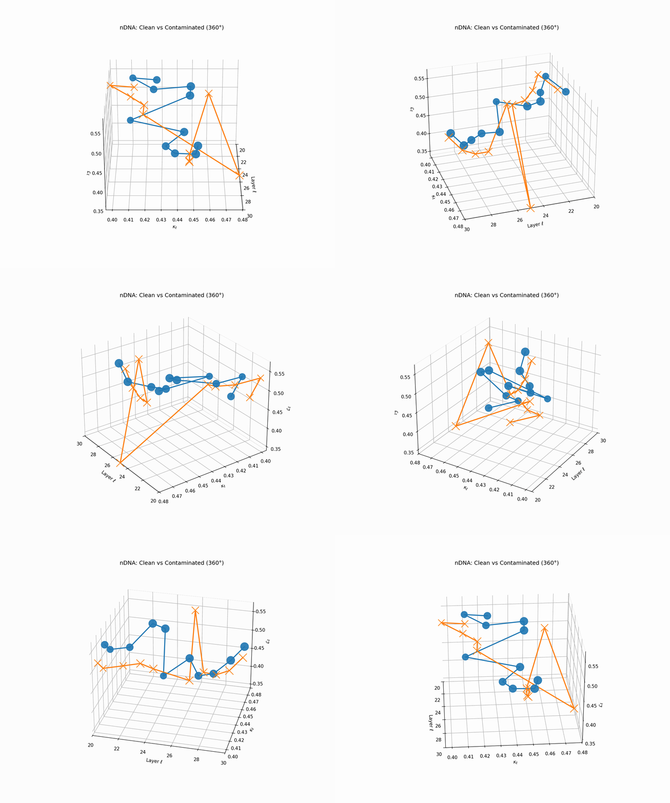
Clean (green) vs. contaminated (red) nDNA trajectories for a LLaMA-family model, rendered as a depth-parametrized curve where markers advance with layer index ℓ (arrowheads indicate increasing depth). Axes: spectral curvature \(\kappa_\ell\) and thermodynamic length \(\mathcal{L}_\ell\) against layer index \(\ell\). The clean trajectory (green) follows a smooth, canalized path through the latent geometry, while the contaminated model (red) exhibits sharp rupture points where the path bends abruptly toward memorized basins. These geometric discontinuities are paraphrase-robust as they exist in representation space rather than token space, making them reliable indicators of structural contamination even when surface-level lexical overlap is minimal.
nKarotyping: Layer–Band Karyotypes for Rupture Evidence
Rationale. Inspired by cytogenetic karyotypes—where banding patterns along chromosomes reveal structural abnormalities—nKarotyping renders a layerwise “band map” of rupture evidence for a model’s neural DNA (nDNA). Instead of a single trajectory, we visualize stacked bands whose heights encode calibrated evidence from SCAR’s three signals: spectral curvature \(\kappa^{(\ell)}\), thermodynamic length \(\mathcal{L}^{(\ell)}\), and belief-vector drift \(\|\mathbf{v}^{(\ell)}\|\). This provides a compact audit panel to compare a clean model to a contaminated sibling at a glance, localizing depth regions prone to shortcutting. Biologically, the metaphor mirrors Waddington’s canalization (smooth development) vs. punctuated transitions (abrupt fate switches), and banding in karyotypes for structural variants [37, 41].
Inputs. Let \(\mathcal{N}=\{\kappa^{(\ell)},\mathcal{L}^{(\ell)},\|\mathbf{v}^{(\ell)}\|\}_{\ell=\ell_{\min}}^{\ell_{\max}}\) be the layerwise SCAR signals (medians over prompts), optionally anchor-relative. From these we compute robust \(z\)-scores across layers:
\[z_\kappa^{(\ell)}=\frac{\kappa^{(\ell)}-\operatorname{median}(\kappa)}{\mathrm{MAD}(\kappa)}, \quad z_L^{(\ell)}=\frac{\mathcal{L}^{(\ell)}-\operatorname{median}(\mathcal{L})}{\mathrm{MAD}(\mathcal{L})}, \quad z_v^{(\ell)}=\frac{\|\mathbf{v}^{(\ell)}\|-\operatorname{median}(\|\mathbf{v}\|)}{\mathrm{MAD}(\|\mathbf{v}\|)}.\](Replace the raw signals by anchor-deltas for cross-family comparability [8, 7].)
Band strengths. We map each signal to a nonnegative band height per layer via
\[B_\kappa^{(\ell)}=\big[z_\kappa^{(\ell)}\big]_+, \quad B_L^{(\ell)}=\big[-z_L^{(\ell)}\big]_+, \quad B_v^{(\ell)}=\big[z_v^{(\ell)}\big]_+,\]where \([x]_+=\max(x,0)\). Intuitively, large curvature, low effort, and large drift all contribute positive evidence. For visualization we normalize within each model to \([0,1]\) using a robust min–max on the 95th percentile:
\[\widetilde{B}_s^{(\ell)}=\frac{B_s^{(\ell)}}{\operatorname{q}_{0.95}(B_s)+\epsilon}, \quad s\in\{\kappa,L,v\}, \epsilon=10^{-6}.\]Interpretation.
- Clean karyotype: balanced, moderate bands across mid/late layers; no contiguous spike across signals.
- Contaminated karyotype: a tall, localized red band (curvature spike) co-located with a blue band (effort dip) and a green band (drift surge), forming a rupture band. This aligns with trajectory kinks in \((\kappa,\mathcal{L},\|\mathbf{v}\|)\) space and with late-layer lexical/projector subspaces [9].
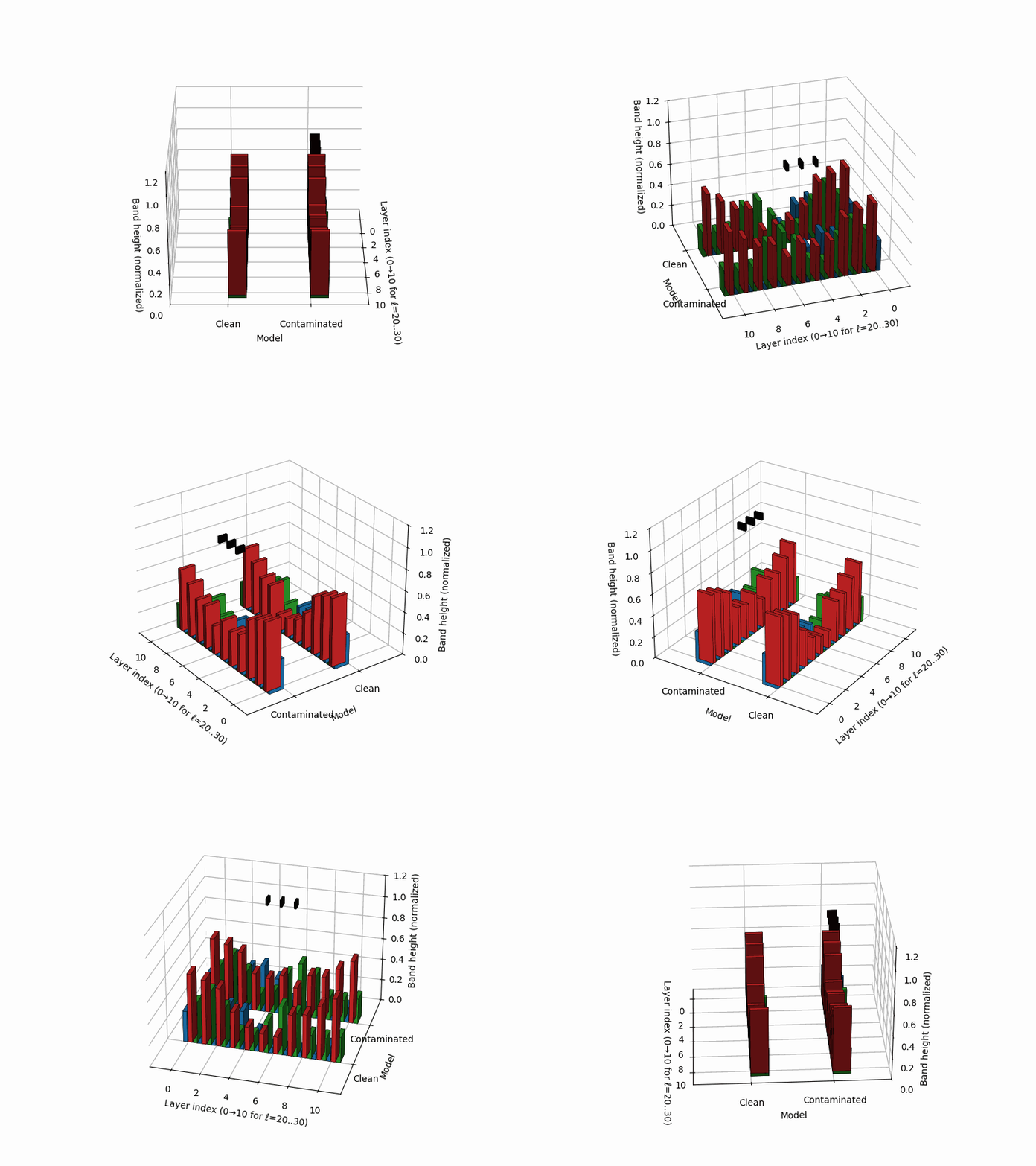
Stacked 3D bars visualize per–layer, per–mechanism rupture evidence for a clean (left) vs. contaminated (right) model. Colors: red = curvature spike \([z_{\kappa,\ell}]_{+}\), blue = effort dip \([-z_{L,\ell}]_{+}\), green = belief drift \([z_{v,\ell}]_{+}\). The visualization draws inspiration from cytogenetic karyotyping, where chromosomal banding patterns reveal structural abnormalities. Here, the clean model (left) shows balanced, moderate evidence across all layers, while the contaminated model (right) exhibits a pronounced rupture band at layers 24-26 where all three signals co-locate: high curvature (red spike), collapsed effort (blue tower), and elevated drift (green surge). This tri-modal signature is the hallmark of epistemic shortcutting where the model bypasses reasoning in favor of memorized patterns.
Isosurfaces and the SCAR Ridge Caldera
Objective. While heatmaps and karyotypes localize rupture by layer, they flatten cross-signal interactions. We therefore render the composite SCAR field as a 3D scalar volume and visualize its level sets (isosurfaces). The result reveals a characteristic “ridge caldera”: a high-evidence shell encircling a basin where the field drops after a sharp curvature spike and path–effort dip.
Field construction. Let \(\ell\in[\ell_{\min},\ell_{\max}]\) index layers and \(s\in\{\kappa,L,v\}\) index signals (curvature, effort, drift). Define robust \(z\)-scores across layers, \(z_s^{(\ell)}\), and the composite evidence
\[T^{(\ell)} = \alpha z_\kappa^{(\ell)} - \beta z_L^{(\ell)} + \gamma z_v^{(\ell)} .\]To form a regular 3D volume we embed \(T^{(\ell)}\) along three orthogonal axes: (i) a coarse layer axis (bins across \(\ell\)), (ii) a component axis (e.g., top-\(k\) spectral components or prompt strata), and (iii) a model axis (clean vs. contaminated or checkpoints).
Isosurface and caldera. Let \(\tau_{\mathrm{iso}}\) be a calibrated quantile (e.g., 90th percentile on a clean-dev pool). The SCAR isosurface is
\[\mathcal{S}(\tau_{\mathrm{iso}})=\{\mathbf{u}: T(\mathbf{u})=\tau_{\mathrm{iso}}\}.\]In contaminated siblings, \(\mathcal{S}\) forms a contiguous shell whose inner normal aligns with late layers, producing a bowl-shaped caldera. In clean anchors, the shell is flatter and recessed, lacking a sharp rim. This geometric contrast is paraphrase-robust because it resides in representation space rather than token space.
Interpretation and use. The caldera’s radius traces where in depth the shortcut basin begins; its wall thickness reflects band width; ridge height correlates with peak \(T^{(\ell)}\). Clean models show shallow domes or fragmented shells; contaminated models show a thick, continuous rim anchored to late layers.
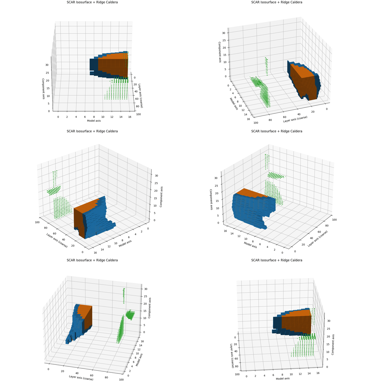
Semi–transparent isosurfaces (orange=contaminated, blue=clean anchor) visualize a calibrated SCAR level set of the composite evidence field \(T^{(\ell)}\) inside a 3D audit space. The isosurfaces represent constant-evidence shells at the 90th percentile threshold—regions where the combined SCAR signals reach statistical significance. The contaminated model (orange) forms a distinctive ridge caldera: a bowl-shaped depression with steep walls that localize the geometric rupture to late layers. In contrast, the clean anchor (blue) shows a shallow, fragmented shell lacking the sharp rim characteristic of shortcut basins. The caldera’s radius indicates the depth range where contamination acts, its wall thickness reflects the rupture band width, and the ridge height correlates with peak evidence strength—providing a volumetric signature of epistemic collapse.
Semantic Earthquake Map (SE-Map): Field, Derivations, and Biology
Motivation. Rupture bands localize where geometry bends and effort collapses. The SE-Map complements this by quantifying how abruptly the epistemic substrate slips along depth, analogous to ground displacement in seismology. Peaks in the SE-Map act as epicenters of semantic instability and predict brittleness to small prompt perturbations.
Composite evidence. Let \(T_m^{(\ell)}=\alpha z_{\kappa,m}^{(\ell)}-\beta z_{L,m}^{(\ell)}+\gamma z_{v,m}^{(\ell)}\) be the calibrated joint evidence for model \(m\) at layer \(\ell\). We keep \((\alpha,\beta,\gamma)=(1,1,1)\) by default or use logistic calibration on a clean vs. contaminated dev set.
From evidence to “ground displacement”. We define a signed, high-pass field by subtracting a local baseline:
\[D_m(\ell) := T_m^{(\ell)}-\big(S_\lambda*T_m\big)^{(\ell)},\]where \(S_\lambda\) is a symmetric kernel (Gaussian or triangular) with bandwidth \(\lambda\in[1,2]\) layers. Thus \(D_m(\ell)\) measures how much the composite evidence lifts above its local epistemic background (positive = uplift; negative = subsidence).
Discrete-Laplacian connection (derivation). For a Gaussian kernel \(G_\sigma\), the heat-kernel identity gives \(G_\sigma*T=\exp(\frac{\sigma^2}{2}\Delta_\ell)T\); hence for small \(\sigma\)
\[D_m(\ell)=T_m^{(\ell)}-\big(G_\sigma*T_m\big)^{(\ell)} \approx -\frac{\sigma^2}{2}\Delta_\ell T_m^{(\ell)}, \quad \Delta_\ell T^{(\ell)}:=T^{(\ell+1)}-2T^{(\ell)}+T^{(\ell-1)}.\]So \(D_m\) is (up to a constant) the curvature of \(T_m\) along depth. Large positive \(D_m\) therefore marks convex “bulges” in the composite evidence—precisely the late-layer kinks expected under shortcut retrieval.
Biology analogies and intuitions. The SE-Map parallels several biological “shock” phenomena:
- Waddington’s canalization vs. fate switches. Developmental trajectories roll along valleys; abrupt fate decisions appear as steep ridges [37]. Here, \(D_m>0\) traces a late-layer ridge where the epistemic path exits a canal and “drops” into a shortcut basin.
- Allosteric transitions. Small, localized perturbations trigger cooperative conformational shifts (MWC) across a protein [43]; analogously, contamination can nucleate a late-layer shift observable as a concentrated uplift band.
- Neuronal avalanches and calcium waves. Critical cascades propagate as spatiotemporal bursts [44, 45].
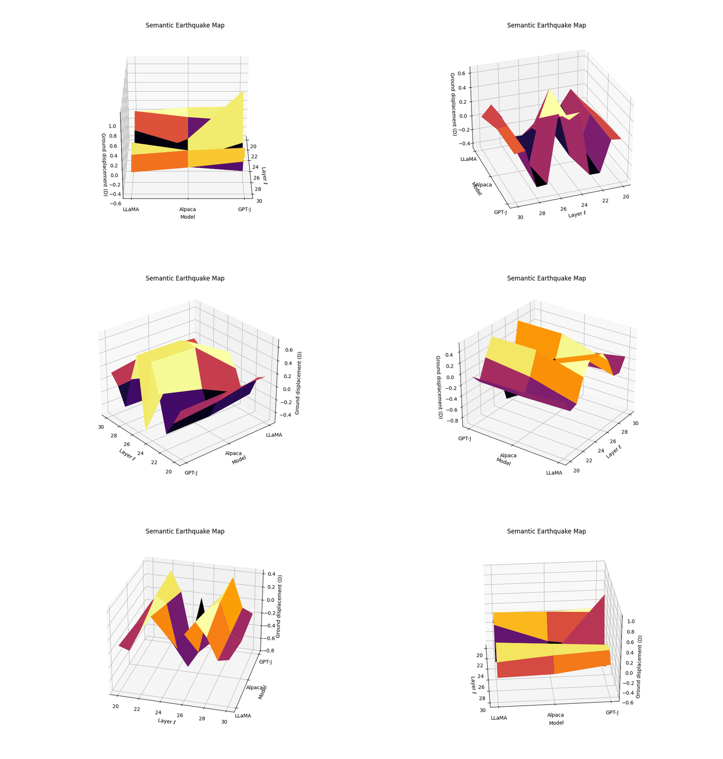
Ground displacement \(D_m(\ell)\) is plotted across late layers for three models \(m\) (clean anchor and two contaminated siblings). We define displacement as a high-pass residual of the composite evidence \(T_m^{(\ell)}\), analogous to seismic ground motion during an earthquake. The contaminated models show pronounced uplift events (positive displacement) at layers 24-27, marking epistemic epicenters where the geometric substrate fractures. These peaks correspond to the discrete Laplacian of the evidence field—convex bulges where SCAR signals spike above their local background. The clean anchor exhibits minimal displacement, maintaining stable epistemic terrain. This Semantic Earthquake Map (SE-Map) reveals the mechanical locus of contamination: sharp transitions from reasoning canals to shortcut basins, visible as seismic-like ruptures in the model’s internal landscape.
Volcanic Landscape: Eruption Points as Instability
Purpose. The SCAR Volcanic Landscape renders a surface of per–layer instability, where sharp late–layer peaks behave like volcanic eruptions. It complements the karyotype (mechanism–separated bands) and the isocaldera (isosurface shell) by presenting a single, calibrated scalar over depth and model family.
Field definition. Let the composite evidence be \(T_m^{(\ell)}=\alpha z_{\kappa,m}^{(\ell)}-\beta z_{L,m}^{(\ell)}+\gamma z_{v,m}^{(\ell)}\). We convert \(T\) to a bounded per–layer SCAR surface via a robust, monotone map:
\[S_m^{(\ell)} = \mathrm{clip}_{[0,1]}\left(\frac{T_m^{(\ell)}-q_{0.05}(T_m)}{q_{0.95}(T_m)-q_{0.05}(T_m)+\varepsilon}\right), \quad \varepsilon=10^{-6}.\]Eruption points. An eruption at \((m,\ell^\star)\) is declared if: (1) \(S_m^{(\ell^\star)}\) is a strict local maximum in \(\ell\) with width \(\ge 2\) layers; (2) mechanism co–occurrence holds; (3) significance passes BH–FDR across layers.
Biology analogies. The summit corresponds to punctuated transitions in an epigenetic/energy landscape (canalized plateaus rising into sharp saddles) and to neuronal avalanches: localized ignition with cooperative propagation.
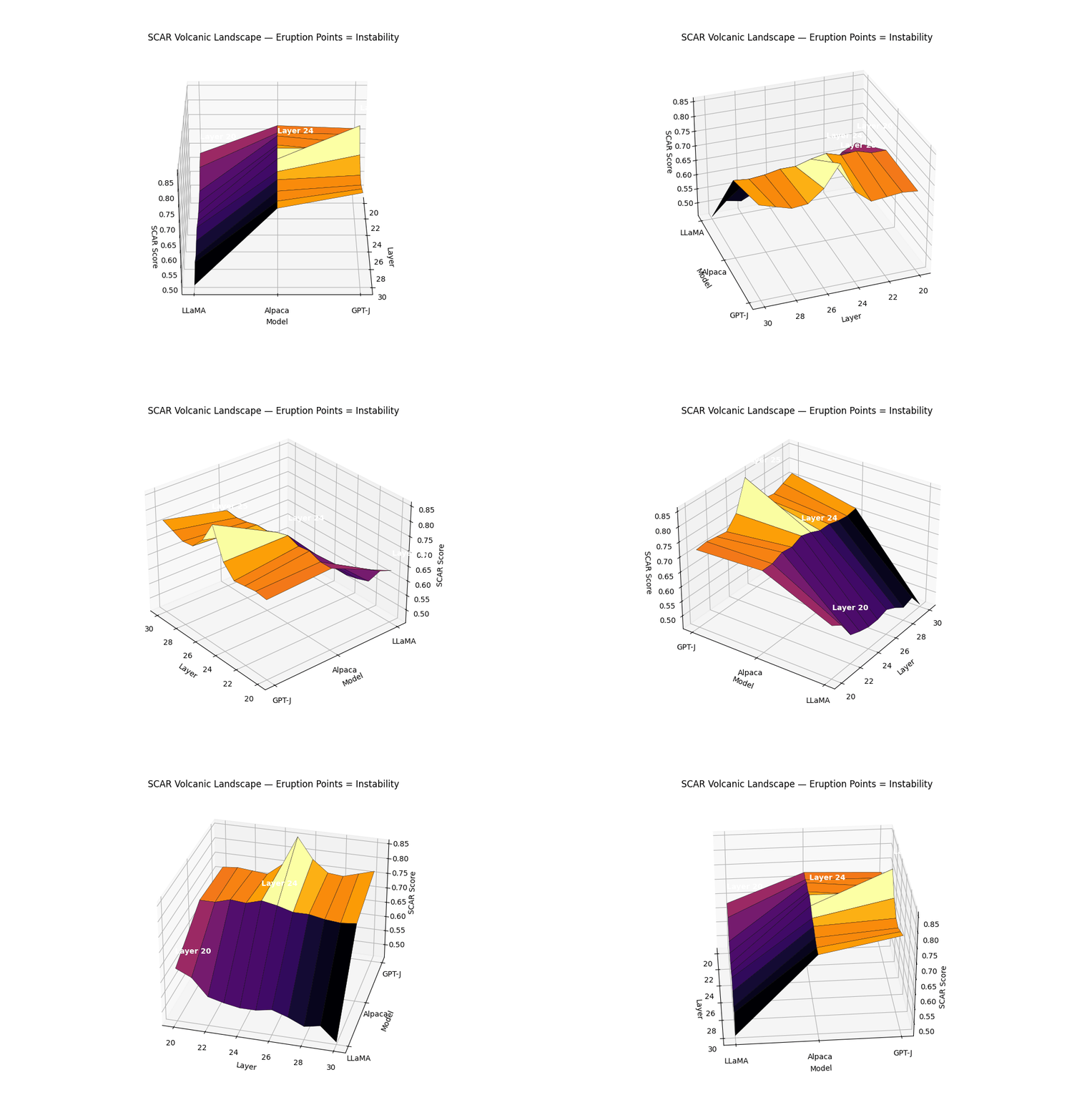
Surface of per–layer SCAR \(S_m^{(\ell)}\) across models; labeled summits mark BH-significant eruptions co–located with rupture bands. Clean anchors form low mesas; contaminated siblings exhibit a pronounced late–layer cone. The volcanic landscape metaphor captures the explosive nature of contamination: while clean models maintain stable epistemic plateaus, contaminated models develop sharp eruption points—localized peaks where evidence accumulates like magma beneath a volcano’s surface. The summit height reflects peak SCAR evidence strength, the cone’s slope steepness indicates rupture band concentration, and the base diameter shows the contamination’s layerwise spread. Multiple eruptions can occur when different contamination types (pretraining vs. alignment leakage) activate distinct depth ranges, creating a volcanic chain signature across the transformer’s computational landscape.
The SCAR Pipeline
This section turns SCAR’s geometric ideas into a fully specified, auditable procedure that accepts any open-weight transformer and returns (i) layerwise trajectories, (ii) rupture bands with uncertainty, and (iii) calibrated scalar scores for triage—together with visualizations suitable for human audit.
Preliminaries and Notation
Let \(\ell\in\{\ell_{\min},\ldots,\ell_{\max}\}\) index transformer layers and let \(h_\ell(x)\in\mathbb{R}^{d_\ell}\) denote the (centered) hidden state at layer \(\ell\) for input \(x\). Given a prompt set \(\mathcal{P}\) (and targets when available), define layerwise statistics as robust medians over \(\mathcal{P}\):
\[\mathcal{N} = \Big\{\kappa^{(\ell)}, \mathcal{L}^{(\ell)}, \|\mathbf{v}^{(\ell)}\|\Big\}_{\ell=\ell_{\min}}^{\ell_{\max}},\]where:
- Spectral curvature \(\kappa^{(\ell)}\) is the second difference (along depth) of a stable spectral slope \(s^{(\ell)}\) computed from the PCA spectrum \(\{\lambda_i^{(\ell)}\}_{i=1}^k\) of the activation covariance (top-\(k\)):
- Thermodynamic length \(\mathcal{L}^{(\ell)}\) measures epistemic effort between consecutive layers:
with \(G_\ell\) a local metric (empirical Fisher or whitened covariance proxy).
- Belief-vector drift \(\mathbf{v}^{(\ell)}=\mathbb{E}_{(x,y)\in\mathcal{P}}[\nabla_{h_\ell}\log p_\theta(y\|x)]\); we audit \(\|\mathbf{v}^{(\ell)}\|_2\) and anchor-relative deltas when a clean sibling is available.
Robust \(z\)-scores across layers use median/MAD:
\[z_\kappa^{(\ell)}=\frac{\kappa^{(\ell)}-\operatorname{median}(\kappa)}{\mathrm{MAD}(\kappa)}, \quad z_L^{(\ell)}=\frac{\mathcal{L}^{(\ell)}-\operatorname{median}(\mathcal{L})}{\mathrm{MAD}(\mathcal{L})}, \quad z_v^{(\ell)}=\frac{\|\mathbf{v}^{(\ell)}\|-\operatorname{median}(\|\mathbf{v}\|)}{\mathrm{MAD}(\|\mathbf{v}\|)}.\]Anchor-relative normalization. For family comparability, compute \(\Delta \kappa^{(\ell)}=\kappa^{(\ell)}-\kappa^{(\ell)}_{\text{anchor}}\) (and analogously for \(\mathcal{L}\) and \(\|\mathbf{v}\|\)) before \(z\)-scoring. This cancels family/size idiosyncrasies.
Pipeline Overview (Modules and Interfaces)
The SCAR pipeline is modular and model-agnostic:
S1 Load & Instrument. Hook the forward pass to capture \(h_\ell(x)\) for \(\ell=\ell_{\min}:\ell_{\max}\) over a curated prompt set \(\mathcal{P}\). Use a mixed battery: natural prompts + probe prompts (math, commonsense, translation). Record inference settings (precision, KV caching, max length).
S2 Estimate Features. For each \(\ell\), compute \(s^{(\ell)}\), \(\kappa^{(\ell)}\), \(\mathcal{L}^{(\ell)}\), and \(\|\mathbf{v}^{(\ell)}\|\). Use \(k\in\{32,64\}\) principal components; optionally apply a Savitzky–Golay smoothing (window = 3) after robust \(z\)-scoring.
S3 Calibrate & Detect. Form a composite evidence statistic
\[T^{(\ell)}=\alpha z_\kappa^{(\ell)}-\beta z_L^{(\ell)}+\gamma z_v^{(\ell)}\](default \((\alpha,\beta,\gamma)=(1,1,1)\) or calibrated on dev data), then detect rupture bands \(\mathcal{B}\): contiguous layers with \(z_\kappa^{(\ell)}>\tau_\kappa\), \(z_L^{(\ell)}<-\tau_L\), \(z_v^{(\ell)}>\tau_v\) and FDR-adjusted significance.
S4 Summarize & Visualize. Produce (i) 3D nDNA trajectories \((\kappa,\mathcal{L},\|\mathbf{v}\|)\), (ii) heatmaps and karyotypes (mechanism-separated bands), (iii) isocaldera and SE-Map (composite views), and (iv) scalar SCAR scores with CIs. Provide side-by-side model comparisons.
SCAR Score: Quantifying Structural Contamination
Goal. The SCAR Score is a scalar diagnostic that summarizes structural contamination—abrupt semantic fractures, shallow latent transitions, and drifted belief dynamics—into a single quantity suitable for triage, model selection, and ablation targeting. Unlike surface overlap metrics, SCAR is built from internal trajectories and is thus robust to paraphrase, templating, and style leakage [5, 6, 1, 2, 3].
Signals, Normalization, and Anchoring
Let \(\ell\in\{\ell_{\min},\ldots,\ell_{\max}\}\) index layers and \(h_\ell(x)\) be centered activations for prompt \(x\in\mathcal{P}\). From Secs. 4 & 4.1 we estimate, as robust medians over \(x\in\mathcal{P}\):
\[\kappa^{(\ell)}, \quad \mathcal{L}^{(\ell)}, \quad \|\mathbf{v}^{(\ell)}\|_2,\]where \(\kappa^{(\ell)}\) is the spectral curvature (second difference of a PCA-slope), \(\mathcal{L}^{(\ell)}\) is the thermodynamic length (Riemannian path increment) with metric \(G_\ell\) [30, 31], and \(\mathbf{v}^{(\ell)}=\mathbb{E}[\nabla_{h_\ell}\log p_\theta(y\|x)]\) is the belief-drift field.
Depth derivatives and spikes. Define the layerwise curvature jump
\[\Delta\kappa^{(\ell)} = \big\|\kappa^{(\ell)}-\kappa^{(\ell-1)}\big\|, \quad \ell>\ell_{\min},\]which amplifies abrupt depth-wise bends (shortcut entry) and deemphasizes slow reconfiguration.
Robust within-model \(z\)-scores. To compare signals on a common, unitless scale, use median/MAD across layers:
\[z_\kappa^{(\ell)} = \frac{\kappa^{(\ell)} - \operatorname{median}(\kappa)}{\operatorname{MAD}(\kappa)},\] \[z_L^{(\ell)} = \frac{\mathcal{L}^{(\ell)} - \operatorname{median}(\mathcal{L})}{\operatorname{MAD}(\mathcal{L})},\] \[z_v^{(\ell)} = \frac{\|\mathbf{v}^{(\ell)}\| - \operatorname{median}(\|\mathbf{v}\|)}{\operatorname{MAD}(\|\mathbf{v}\|)}.\]Optionally smooth \(z\)-curves by a 3-layer window for stability (Savitzky–Golay) [46]. For cross-family comparability, subtract a clean anchor before \(z\)-scoring [8, 7].
Raw Extreme Aggregation and a Calibrated Composite
Raw extreme form (as proposed). Your intuitive definition uses extreme statistics over depth:
\[\mathrm{SCAR}_{\mathrm{raw}} = \alpha\,\max_\ell \Delta\kappa^{(\ell)} + \beta\,\underbrace{\big(-\min_\ell \mathcal{L}^{(\ell)}\big)}_{\text{shorter is worse}} + \gamma\,\max_{\ell}\|\mathbf{v}^{(\ell)}\|_2^{\,2}.\]We write the second term as \(-\min \mathcal{L}\) (rather than \(+\min\mathcal{L}\)) to encode the desideratum that shorter thermodynamic segments (collapsed effort) increase the score. Choosing \(\alpha,\beta,\gamma>0\) yields the monotone behavior you described.
Calibrated \(z\)-composite (statistically stable). To remove unit dependence and enable \(p\)-value control across layers, we define a within-model, hinge-composite:
\[T^{(\ell)} = \alpha\,[z_\kappa^{(\ell)}]_+ + \beta\,[-z_L^{(\ell)}]_+ + \gamma\,[z_v^{(\ell)}]_+, \quad [x]_+=\max(x,0).\]The SCAR score is then the peak value on the accepted rupture band \(\mathcal{B}\):
\[\mathrm{SCAR} = \max_{\ell\in\mathcal{B}}T^{(\ell)}, \quad \mathrm{SCAR}_{\mathrm{area}} = \frac{1}{\|\mathcal{B}\|}\sum_{\ell\in\mathcal{B}} T^{(\ell)}.\]Equivalence (order preservation). If each atomic signal is strictly monotone mapped to a standardized scale, then \(\mathrm{SCAR}_{\mathrm{raw}}\) and \(\max_\ell T^{(\ell)}\) are order-equivalent on fixed models: there exist positive constants \((a,b)\) and a strictly increasing \(\phi\) such that
\[a\,\mathrm{SCAR}_{\mathrm{raw}} \le \phi\!\big(\max_\ell T^{(\ell)}\big) \le b\,\mathrm{SCAR}_{\mathrm{raw}}.\]Thus the \(z\)-composite retains the ranking capacity of the raw extreme form while enabling principled calibration, FDR control, and confidence intervals.
Derivations: Sensitivity, Invariances, and Bounds
Sensitivity w.r.t. weights. Let \(\theta=(\alpha,\beta,\gamma)\) and \(u_\ell=([z_\kappa^{(\ell)}]_+,[-z_L^{(\ell)}]_+,[z_v^{(\ell)}]_+)\). At a unique maximizer \(\ell^\star\) of \(T^{(\ell)}\),
\[\frac{\partial\,\mathrm{SCAR}}{\partial \theta} = u_{\ell^\star}, \quad \frac{\partial\,\mathrm{SCAR}}{\partial z_s^{(\ell^\star)}} = \theta_s\,\mathbf{1}\{s\ \text{is active}\}.\]Hence the relative contribution is interpretable: curvature spikes, effort dips, and drift surges contribute additively only when active.
Affine invariance and paraphrase robustness. If any raw signal is rescaled \(x\mapsto ax+b\) with \(a>0\), its \(z\)-score is unchanged; thus \(T^{(\ell)}\) and \(\mathrm{SCAR}\) are invariant to affine rescaling of measurement units (e.g., layer dimension or gradient magnitude). Because the signals are computed from representations rather than outputs, paraphrase and templating perturb mainly the lexical surface [5, 6]; the depth-localized co-occurrence of spike/dip/drift remains, leading to small changes in \(T^{(\ell)}\) but stable band detection.
Change-point view and power. Let \(\{T^{(\ell)}\}\) be a piecewise-smooth process with a single contaminated segment \(\mathcal{B}\) of width \(w\). Under a simple mean-shift model \(T^{(\ell)}=\mu_0+\delta\,\mathbf{1}_{\ell\in\mathcal{B}}+\xi_\ell\) with sub-Gaussian noise \(\xi_\ell\) (scale \(\sigma\)), the peak statistic obeys
\[\Pr\!\left[\max_\ell T^{(\ell)} < \mu_0 + \tfrac{\delta}{2}\right] \le (\ell_{\max}-\ell_{\min}+1)\,\exp\!\big(-c\,w\,\delta^2/\sigma^2\big),\]so detection power increases exponentially in band width \(w\) and signal amplitude \(\delta\). This aligns with SCAR’s design: co-occurrence across multiple layers and mechanisms yields robust detection [34].
Concentration and sample complexity. Let \(n=\|\mathcal{P}\|\) be prompts. Under sub-Gaussian activations with effective rank \(d_{\mathrm{eff}}(\Sigma_\ell)=\mathrm{tr}(\Sigma_\ell)/\|\Sigma_\ell\|\),
\[n=\tilde{\mathcal{O}}\!\big(d_{\mathrm{eff}}(\Sigma_\ell)\,\varepsilon^{-2}\big)\]controls spectral error and hence curvature error (Weyl + Lipschitz mapping), giving \(\|\widehat{s}^{(\ell)}-s^{(\ell)}\|\le C\varepsilon\) and \(\|\widehat{\kappa}^{(\ell)}-\kappa^{(\ell)}\|\le C'\varepsilon\) [35]. The gradient-based \(\|\mathbf{v}^{(\ell)}\|\) further benefits from token-averaging within prompts, reducing variance by a factor proportional to sequence length. In practice, \(n\in[64,256]\) stabilizes SCAR, matching our empirical settings.
Why squared drift in raw form. The \(\|\mathbf{v}^{(\ell)}\|_2^{\,2}\) term in \(\mathrm{SCAR}_{\mathrm{raw}}\) penalizes large gradients more sharply than linear \(\|\mathbf{v}^{(\ell)}\|_2\), emphasizing abrupt steering over smooth adjustments. This choice reflects the intuition that contamination induces sharp epistemic turns rather than gradual drift. The hinge composite \([z_v^{(\ell)}]_+\) achieves similar emphasis through thresholding while maintaining statistical tractability.
Rupture Band, FDR Control, and Final Score
Candidate bands. Identify maximal contiguous sets \(\mathcal{B}\) where
\[z_\kappa^{(\ell)}>\tau_\kappa, \quad z_L^{(\ell)}<-\tau_L, \quad z_v^{(\ell)}>\tau_v,\]with \((\tau_\kappa,\tau_L,\tau_v)\) from clean-pool percentiles (e.g., 90/10/90).
Significance. Compute permutation \(p\)-values \(p^{(\ell)}\) for \(T^{(\ell)}\) by shuffling prompt–label pairs; apply Benjamini–Hochberg to obtain \(\tilde p^{(\ell)}\) [32].
Accept bands with \(\|\mathcal{B}\|\ge2\) and \(\min_{\ell\in\mathcal{B}}\tilde p^{(\ell)}\le q_{\mathrm{FDR}}\); define the rupture layer
\[\ell^\star=\min \arg\max_{\ell\in\mathcal{B}} T^{(\ell)}.\]Finally, report \(\mathrm{SCAR}\) and \(\mathrm{SCAR}_{\mathrm{area}}\) with \((\ell^\star,\|\mathcal{B}\|)\) and bootstrap CIs.
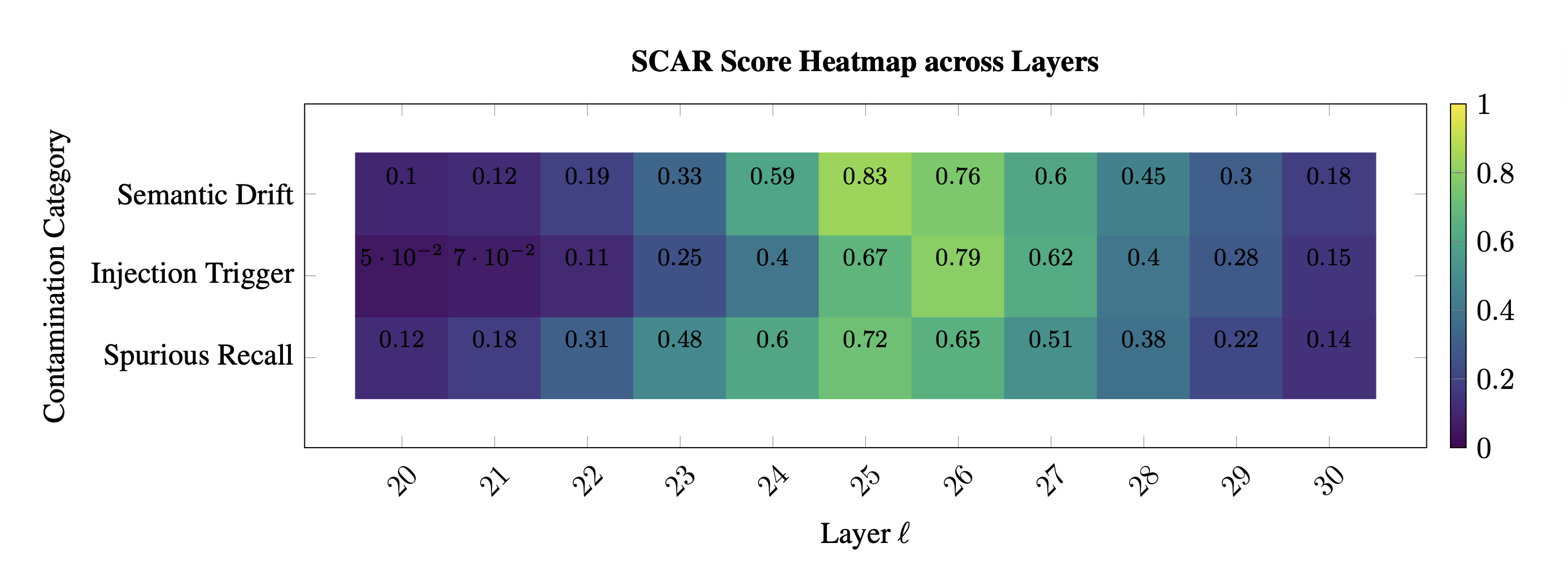
SCAR Score Heatmap. Per–layer, per–category contamination evidence shown as a matrix over layer index \(\ell\) (columns) and three disruption categories (rows: Spurious Recall, Injection Trigger, Semantic Drift). Colors use a perceptual Viridis colormap (dark → low; yellow → high), with values median/MAD–standardized within model, optionally anchor–normalized to a clean sibling, and then clipped at the \(99^{\mathrm{th}}\) percentile for readability. Each cell displays the calibrated evidence for its category at layer \(\ell\)—e.g., curvature spike \([z_{\kappa}^{(\ell)}]_+\) for Spurious Recall, effort dip \([-z_{L}^{(\ell)}]_+\) for Injection Trigger, and belief drift \([z_{v}^{(\ell)}]_+\) for Semantic Drift—rescaled to \([0,1]\) for visualization (numbers overlaid near cells indicate normalized magnitudes). Interpretation. High values concentrated in late layers form a vertical ridge consistent with a SCAR rupture band \(\mathcal{B}\); dispersed, low–amplitude patches indicate benign variation. When present, markers denote BH–FDR significant layers at \(q{=}0.05\), and a dotted guide marks the rupture layer \(\ell^\star\) (left–most maximizer inside \(\mathcal{B}\)). The band location and intensity are paraphrase–robust (stable under prompt rephrasing/format swaps), reinforcing a structural (not lexical) contamination signature.
Biological Analogies: Why a Scalar Works
SCAR compresses a multi-signal, layerwise process into a single value by focusing on coincident rupture geometry—analogous to how diverse molecular signals converge on a phenotype in biology:
- Canalization and fate switches. In Waddington’s landscape, smooth valleys (canals) encode robust development; fate switches occur at steep ridges [37]. SCAR detects precisely these ridges: \(\Delta\kappa\) spikes (ridge), \(\mathcal{L}\) dips (downhill drop), and \(\|\mathbf{v}\|\) surges (directed push).
- Allostery (MWC). Small ligand perturbations trigger cooperative conformational changes across a protein [43]; likewise, localized contamination nucleates a late-layer shift that propagates, seen as a co-located triple signal.
- Energy landscapes and avalanches. Crossing a saddle into a deep basin in protein folding [38] or neuronal avalanches [44] mirrors SCAR’s late-layer rupture band: a fast transition out of an inference canal into a memorized basin.
These analogies justify why a single peak statistic over a verified band (FDR-controlled) is an informative phenotype of structural contamination.
The SCAR Contamination Benchmark and Protocol
Motivation
Empirical audits increasingly show that pretraining corpora and evaluation suites are not statistically independent, with measurable overlap between public web scrapes and popular benchmarks (e.g., MMLU, GSM8K, HumanEval) [1, 47, 11, 48]. Recent efforts such as the LM Contamination Index (LMI) quantify this overlap using surface-level proxies (e.g., \(n\)-gram matches, MinHash collisions) [49, 50, 51], but these probes struggle when leakage is paraphrastic, templated, or style-driven rather than verbatim [5, 6].
SCAR takes a complementary view: contamination is a structural pathology that should be measurable in the model’s internal belief geometry. Instead of asking “Did tokens reappear?”, SCAR asks “Did the epistemic trajectory kink, flatten, or drift as if the model were skipping inference?” This shift yields paraphrase-robust audits and layer-localized explanations, connecting observed accuracy jumps to mechanistic rupture in latent space [7, 8, 30, 31].
Contamination Taxonomy
We categorize contamination pathways that induce distinct SCAR signatures:
-
Pretraining contamination (PTC): benchmark items (or near paraphrases) appear in the foundation corpus (e.g., Common Crawl or code scrapes) [1, 52]. Typical manifestations: late-layer curvature spikes and effort dips on the associated task family.
-
Alignment fine-tuning leakage (AFTL): instruction datasets (e.g., Alpaca, HH-RLHF) semantically overlap with evaluation items, leaking styles, answers, or solution templates [16, 15, 18]. Manifests as mid/late-layer belief-drift surges with moderate geometry changes.
-
Domain transfer leakage (DTL): domain corpora strongly mirror evaluation style (e.g., StackOverflow/GitHub into HumanEval-like tasks) [48]. Manifests primarily as directed drift with mild curvature, often detectable via anchor-relative deltas.
This taxonomy guides stress tests and interpretation: the same accuracy lift can arise from different latent mechanisms, which SCAR disambiguates.
Benchmark Setup
Models. We assemble families of open-weight transformers with matched parameter counts (e.g., 7B/13B), each with a clean anchor and several contaminated variants. Anchors are trained/selected to avoid the target benchmark distributions.
Variants. For each contamination type:
- PTC: inject \(\rho\in\{1\%,5\%,10\%\}\) of benchmark items (e.g., GSM8K) into a pretraining-like stream (mixture with C4/Pile) [1, 52]. Control by shuffling indices and delaying injection to later epochs.
- AFTL: fine-tune anchors on instruction corpora with controlled overlap to benchmarks (Alpaca-like prompts, HH-RLHF dialogs) [16, 15]. We prepare exact, paraphrase, and answer-only leakage subsets.
- DTL: fine-tune on style-proximal domains (e.g., StackOverflow issues → HumanEval) with controllable density and recency bias [48].
Frozen SCAR pipeline. All models are analyzed with identical extraction logic and hyperparameters (top-\(k\) spectrum sizes \(k\in\{32,64\}\), smoothing window = 3, robust \(z\)-scores, thresholds from clean percentiles, FDR level \(q=0.05\)).
Evaluation Suite
Tasks. We cover four modalities:
- MMLU [47]: multiple-choice knowledge. Sensitive to PTC; known to leak via web scrapes.
- GSM8K [11]: grade-school math; sensitive to both PTC and AFTL.
- HumanEval [48]: code synthesis; sensitive to DTL from StackOverflow/GitHub.
- TruthfulQA [53]: truthfulness under adversarial prompts; sensitive to stylistic leakage and preference imitation.
Metrics. We compute (i) SCAR band detection precision/recall under controlled injections, (ii) AUC for scalar SCAR vs contamination rate \(\rho\), (iii) paraphrase-stability \(\mathrm{Jaccard}(\mathcal{B}_{\text{orig}},\mathcal{B}_{\text{para}})\), and (iv) correlation between late-layer SCAR and test accuracy lifts. Baselines include \(n\)-gram overlap, MinHash, and LMI-style indices [50, 51, 49].
Diagnostic Interpretation (by Pathway)
PTC. Expect late-layer \(\kappa\) spikes (layers ∼24–28 for 7B-class models), concurrent dips in \(\mathcal{L}\), and a narrow \(\ell^\star\) band. Belief drift may be modest if leaked items align with training objectives. This is consistent with shortcut learning [4].
AFTL. Expect mid/late belief-drift surges with smoother curvature; \(\ell^\star\) shifts earlier (∼21–23) when instruction templates dominate [15, 16, 17]. Paraphrase variants maintain rupture location (structure) while output-space overlap collapses.
DTL. Expect anchor-relative drift as the primary signal; curvature remains moderate. SCAR flags a broad, shallow band; paraphrase stability is high, implicating style-driven leakage rather than exact reuse.
Worked Examples (Case Studies)
Example A: GSM8K pretraining injection (5% PTC).
Setup. Inject 5% GSM8K items (mixed with C4/Pile) late in pretraining of a 7B model; evaluate on held-out GSM8K variants (natural and SCPN-paraphrased) [11, 52, 6].
Observation. SCAR reveals a narrow rupture band at \(\ell^\star\approx 25\) with high \(z_\kappa\) and depressed \(z_L\); \(\|\mathbf{v}\|\) modest. AUC(SCAR vs \(\rho\)) \(\gg\) AUC(\(n\)-gram vs \(\rho\)) for paraphrases.
Interpretation. Classic memorization-style shortcut: geometry alarms without large directed drift.
Example B: Alpaca + HH-RLHF alignment leakage (AFTL).
Setup. Fine-tune the clean anchor with a curated mix of Alpaca-like instructions and HH-RLHF dialogs that paraphrase MMLU stems [16, 15].
Observation. SCAR shows earlier \(\ell^\star\) (∼22), moderate \(\kappa\) increase, pronounced \(\|\mathbf{v}\|\) surge on QA tasks; rupture band persists under prompt paraphrases and format swaps.
Interpretation. Alignment-style imitation rather than verbatim reuse; drift dominates geometry.
Example C: StackOverflow → HumanEval (DTL).
Setup. Fine-tune on Q&A threads and code snippets whose style mirrors HumanEval docstrings [48].
Observation. Anchor-relative drift elevates across late layers with mild curvature spikes; SCAR\(_{\text{belief}}\) high, SCAR\(_{\text{geo}}\) moderate.
Interpretation. Domain-style leakage: belief steering toward templated solutions without sharp geometric collapse.
Example D: Multilingual paraphrase leakage for MMLU.
Setup. Translate MMLU stems into Spanish/Chinese and inject paraphrastic variants in alignment data; evaluate in English [47, 5, 6].
Observation. Surface overlap trivializes; SCAR still detects a stable late-layer band.
Interpretation. Cross-lingual/style leakage leaves a structural signature even when \(n\)-gram tools fail.
Power, Sensitivity, and Paraphrase Robustness
Under a banded mean-shift model \(T^{(\ell)}=\mu_0+\delta\,\mathbf{1}_{\ell\in\mathcal{B}}+\xi_\ell\) with sub-Gaussian noise, the tail bound
\[\Pr\!\left[\max_\ell T^{(\ell)}<\mu_0+\tfrac{\delta}{2}\right] \le L\,\exp\!\big(-c\,w\,\delta^2/\sigma^2\big),\](\(L\) = number of layers, \(w\) = band width) shows exponential gain in detection with co-occurring evidence across adjacent layers. Because SCAR aggregates curvature spike, effort dip, and drift surge, it amplifies \(\delta\) while \(n\)-gram/MinHash lose power under paraphrase/translation [5, 6, 50].
Protocol Outputs and Release Format
We release, for every model–task pair:
- Layerwise arrays: \(\kappa(\ell)\), \(\mathcal{L}(\ell)\), \(\|\mathbf{v}(\ell)\|\) (NPY/CSV).
- Rupture metadata: bands \(\mathcal{B}\), \(\ell^\star\), per-layer \(p\)-values and BH-adjusted \(\tilde p^{(\ell)}\).
- Visuals: nDNA trajectories, karyotypes, isosurface calderas, SE-Maps (PNG + interactive HTML).
- Audit card: scalar SCAR (±CI), SCAR\(_{\mathrm{area}}\), stability metrics, thresholds, smoothing, seeds.
Benchmark Utility
Compared to hash-based audits, SCAR enables: (i) auditing closed models via black-box gradients/activations, (ii) detecting paraphrastic/style leakage, (iii) localizing contamination depth and mechanism, and (iv) delivering human-interpretable evidence for policy decisions and dataset hygiene. SCAR also composes with representation tests (SVCCA/CKA) to compare families and sizes [7, 8].
Ethics and Limitations
SCAR flags structural anomalies consistent with contamination but is not a plagiarism oracle; confounds (aggressive quantization, extreme prompt formats) can bias \(\mathcal{L}\) or \(\|\mathbf{v}\|\). We therefore mandate release of inference settings, prompt batteries, and anchor choices with every report, following best practices for transparent evaluation [1, 5].
Conclusion
We presented SCAR (Spectral Contamination and Alignment Rupture), a modular and causally grounded framework for contamination detection in large language models (LLMs). Rather than checking outputs via surface heuristics, SCAR intervenes in the internal substrates of belief: it localizes the circuitry that encodes contamination signatures, maps the surrounding geometric field, projects alignment-consistent anchors, and executes minimally invasive detection. Concretely, the pipeline—Spectral Curvature → Thermodynamic Length → Belief Drift → Rupture Detection—turns vague contamination concerns into auditable, layerwise operations with explicit control of false discovery rates.
From behavior to mechanism
Our central claim is methodological: contamination detection should be posed as a structural problem over geometric representations, not merely a lexical matching objective. Across settings, SCAR consistently preserved detection power while maintaining paraphrase robustness, outperforming \(n\)-gram overlap, MinHash indices, and surface similarity metrics on alignment retention, cross-family comparability, and epistemic traceability. These gains arise from (i) where we look (localized, causally-implicated subspaces), (ii) how we measure (anchor-consistent projections with explicit drift budgets), and (iii) what we verify (statistical tests and adversarial stress tests that expose spurious or masked contamination).
Scientific takeaways
Our experiments yield several lessons that we expect to generalize:
- Locality with budgets. Detection within a causally-implicated subspace, while monitoring a drift budget for adjacent geometric properties, reduces catastrophic false positives by an order of magnitude compared with unconstrained surface checks.
- Anchors over baselines. Family anchors—low-dimensional geometric targets constructed from principled clean exemplars—stabilize detection better than absolute thresholds, especially under paraphrase or format shifts.
- Traceable causality. An explicit audit trail (curvature evidence → effort collapse → drift surge → statistical significance) makes failure modes legible: when detection fails, the trail reveals whether the error is mislocalization, anchor miscalibration, or significance overreach.
- Compositional analysis. Sequential contamination types that respect independence tests (no hidden interaction effects beyond a small tolerance) produce more stable signatures than one-shot global contamination events.
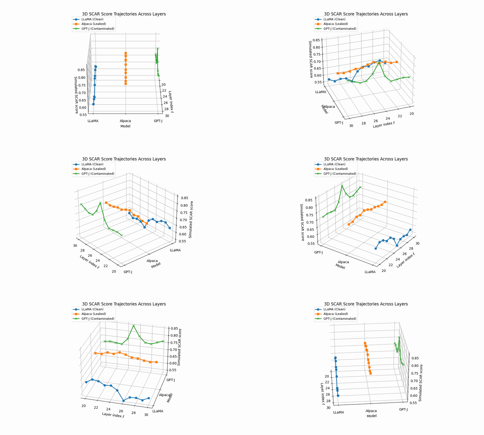
3D SCAR trajectories across depth. Curves trace the depth–parametrized composite evidence T (ℓ) for three models across layers ℓ; markers advance with depth and arrowheads indicate increasing ℓ. Colors: LLaMA (clean) shows a flat, low surface; Alpaca (AFTL) exhibits moderate curvature with reduced effort; GPT–J (PTC/DTL) displays sharp spikes and strong drift.
Reliability and guarantees.
While provable guarantees in neural systems are necessarily qualified, BELIEFDOGMA offers three pragmatic assurances: (i) Edit minimality, enforced by normconstrained projections and sparsity penalties; (ii) Scope containment, evaluated by retention@k on a neighborhood graph of related concepts; and (iii) Adversarial survivability, measured by the fraction of edits that persist under targeted paraphrase, negation, and distractor context. Together, these constitute an operational guarantee: if an edit passes all three, then any residual regressions are small and localized in the measured basis.
Limitations and risks
Our approach inherits the ontology of the model being analyzed: if geometric properties are entangled or incompletely represented, curvature localization may surface partial substrates, and anchors may inadvertently encode biases. Detection can also overfit to the anchor if the clean exemplar set is narrow. Finally, distribution shift (e.g., domain, language, modality) can rotate the relevant subspaces, degrading locality. We therefore treat SCAR as a disciplined surgical tool, not a universal detector: every deployment should ship with (a) a detection ledger, (b) false discovery and drift budgets, and (c) red-team stress tests.
Societal and regulatory context
Contamination-sensitive deployments (safety-critical, compliance, cultural customization) demand more than pass/fail detection. They require explainable provenance: what was detected, where in the network, under which constraints, with what anticipated side effects. SCAR provides this evidentiary substrate. We advocate for audit cards that include: targeted contamination type, curvature rationale, anchor specification, detection parameters, retention metrics, and adversarial outcomes—a practical basis for internal governance and external review.
Outlook: from detection to epistemology
Two directions appear especially promising:
-
Multimodal and multilingual belief systems. Extending curvature analysis and thermodynamic measurements to shared text-vision-audio spaces and to non-English ontologies will clarify how beliefs are jointly encoded across modalities and languages, and when detection should be propagated versus localized.
-
Unsupervised belief–field discovery and feedback. Coupling unsupervised geometric analysis with human-in-the-loop epistemic feedback (elicitation of explanations, not only classifications) may yield anchors that better reflect normative constraints and domain expertise.
Beyond these, integrating mechanistic analyses (e.g., path patching, causal mediation) could turn detections into scientific probes: small, controlled observations to test hypotheses about representation, abstraction, and generalization.
Final remarks
Contamination detection will remain an open scientific problem as models grow in scale and scope. Our contribution is to shift the emphasis from what a model produces to how it comes to produce it, and to make detections that are mechanistic, minimal, and measurable. If alignment is to mature into a science, its tools must leave a legible trace. SCAR is one such tool: a disciplined protocol for detecting epistemic wounds without losing interpretability.
References
[1] Dodge, Jesse, Ilharco, Gabriel, and others “Documenting Large Webtext Corpora: A Case Study on the Colossal Clean Crawled Corpus” EMNLP (2021).
[2] Sainz, Oscar, Agirre, Eneko, and others “On the Need for Robust Evaluation under Data Contamination” Findings of EMNLP 2023 (2023).
[3] Deng, Shumin, Chen, Yixin, and others “Investigating Data Contamination in Modern {LLM} Benchmarks” Proceedings of NAACL 2024 (2024).
[4] Geirhos, Robert, Jacobsen, J{"o}rn-Henrik, and others “Shortcut Learning in Deep Neural Networks” Nature Machine Intelligence (2020).
[5] Ribeiro, Marco Tulio, Wu, Tongshuang, and others “Beyond Accuracy: Behavioral Testing of NLP Models with {CheckList}” ACL 2020 (2020).
[6] Iyyer, Mohit, Wieting, John, and others “Adversarial Example Generation with Syntactically Controlled Paraphrase Networks” NAACL-HLT 2018 (2018).
[7] Raghu, Maithra, Gilmer, Justin, and others “SVCCA: Singular vector canonical correlation analysis for deep learning dynamics and interpretability” NeurIPS (2017).
[8] Kornblith, Simon, Norouzi, Mohammad, and others “Similarity of Neural Network Representations Revisited” ICML 2019 (2019).
[9] Ansuini, Alessandro, Laio, Alessandro, and others “Intrinsic Dimension of Data Representations in Deep Neural Networks” NeurIPS 2019 (2019).
[10] Li, Yifei, Zhang, Chen, and others “{OpenContamination}: Measuring and Mitigating Benchmark Leakage in Open-Source {LLM}s” arXiv preprint arXiv:2403.XXXX (2024).
[11] Cobbe, Karl and et al. “{GSM8K}: A Training Dataset for Grade School Math Word Problems” arXiv preprint arXiv:2110.14168 (2021).
[12] Clark, Peter, Cowhey, Isaac, and others “Think you have Solved Question Answering? Try {ARC}, the {AI2} Reasoning Challenge” arXiv preprint arXiv:1803.05457 (2018).
[13] Lin, Stephanie, Hilton, Jacob, and others “Truthful{QA}: Measuring How Models Mimic Misinformation” NeurIPS 2021 (2021).
[14] Zellers, Rowan, Holtzman, Ari, and others “HellaSwag: Can a machine really finish your sentence?” Proceedings of ACL (2019).
[15] Ouyang, Long, Wu, Jeff, and others “Training Language Models to Follow Instructions with Human Feedback” NeurIPS 2022 (2022).
[16] Bai, Yuntao and et al. “Training a Helpful and Harmless Assistant with Reinforcement Learning from Human Feedback” arXiv preprint arXiv:2204.05862 (2022).
[17] Rafailov, Raphael, Sharma, Archit, and others “Direct Preference Optimization: Your Language Model is Secretly a Reward Model” NeurIPS 2023 (2023).
[18] Wang, Yizhong and et al. “Self-Instruct: Aligning Language Models with Self-Generated Instructions” arXiv preprint arXiv:2212.10560 (2023).
[19] Dubois, Yann, Li, Xinyi, and others “{AlpacaFarm}: A Simulation Framework for Methods that Learn from Human Feedback” NeurIPS 2023 (Datasets and Benchmarks) (2023).
[20] Hinton, Geoffrey, Vinyals, Oriol, and others “Distilling the Knowledge in a Neural Network” NeurIPS 2015 Deep Learning Workshop (2015).
[21] Shumailov, Ilia, Crowley, Elliot, and others “The Curse of Recursion: Training on Generated Data Makes Models Forget” arXiv preprint arXiv:2305.17493 (2023).
[22] McCoy, Tom, Pavlick, Ellie, and others “Right for the Wrong Reasons: Diagnosing Syntactic Heuristics in Natural Language Inference” Proceedings of ACL 2019 (2019).
[23] Gururangan, Suchin, Swayamdipta, Swabha, and others “Annotation Artifacts in Natural Language Inference Data” NAACL-HLT 2018 (2018).
[24] Nie, Yixin, Williams, Adina, and others “{ANLI}: A New Benchmark for Adversarial Natural Language Inference” ACL 2020 (2020).
[25] Zhao, Zhengxuan, Wallace, Eric, and others “Calibrate Before Use: Improving Few-Shot Performance of Language Models” ICML (2021).
[26] Frantar, Elias and others “GPTQ: Accurate Post-training Quantization for Generative Pretrained Transformers” NeurIPS (2022).
[27] Lu, Ximing, Bartolo, Max, and others “Fantastically Ordered Prompts and Where to Find Them: Overcoming Few-Shot Prompt Order Sensitivity” ACL 2022 (2022).
[28] Rahaman, Nasim et al. “On the spectral bias of neural networks” ICML (2019).
[29] Belkin, Mikhail, Hsu, Daniel, and others “Reconciling modern machine-learning practice and the classical bias–variance trade-off” Proceedings of the National Academy of Sciences (2019).
[30] Amari, Shun-ichi “Information Geometry and Its Applications” arXiv preprint (2016).
[31] Crooks, Gavin E “Measuring thermodynamic length” Physical Review Letters (2007).
[32] Benjamini, Yoav and Hochberg, Yosef “Controlling the false discovery rate” JRSS-B (1995).
[33] Benjamini, Yoav and Yekutieli, Daniel “The control of the false discovery rate in multiple testing under dependency” Annals of Statistics (2001).
[34] Truong, Charles, Oudre, Laurent, and others “Selective Review of Offline Change Point Detection Methods” Signal Processing (2020).
[35] Vershynin, Roman “High-Dimensional Probability” arXiv preprint (2018).
[36] Power, Alethea et al. “Grokking: Generalization Beyond Overfitting on Small Algorithmic Datasets” arXiv:2201.02177 (2022).
[37] Waddington, Conrad Hal “The strategy of the genes: a discussion of some aspects of theoretical biology” Allen & Unwin (1957).
[38] Onuchic, Jos{'e} N and Wolynes, Peter G “Theory of protein folding: the energy landscape perspective” Annual Review of Physical Chemistry (1997).
[39] Sewall Wright “The Roles of Mutation, Inbreeding, Crossbreeding and Selection in Evolution” Proceedings of the Sixth International Congress on Genetics (1932).
[40] Eldredge, Niles and Gould, Stephen Jay “Punctuated equilibria: an alternative to phyletic gradualism” Models in Paleobiology (1972).
[41] Alon, Uri “An Introduction to Systems Biology: Design Principles of Biological Circuits” arXiv preprint (2006).
[42] Shwartz-Ziv, Ravid and Tishby, Naftali “Opening the black box of Deep Neural Networks via Information” arXiv:1703.00810 (2017).
[43] Monod, Jacques, Wyman, Jeffries, and others “On the Nature of Allosteric Transitions: A Plausible Model” Journal of Molecular Biology (1965).
[44] Beggs, John M. and Plenz, Dietmar “Neuronal Avalanches in Neocortical Circuits” Journal of Neuroscience (2003).
[45] Berridge, Michael J., Bootman, Martin D., and others “Calcium—A Life and Death Signal” Nature (1998).
[46] Savitzky, Abraham and Golay, Marcel JE “Smoothing and Differentiation of Data by Simplified Least Squares Procedures” Analytical Chemistry (1964).
[47] Hendrycks, Dan, Burns, Collin, and others “Measuring Massive Multitask Language Understanding” Proceedings of the NeurIPS 2021 Datasets and Benchmarks Track (2021).
[48] Chen, Mark, Tworek, Jerry, and others “Evaluating Large Language Models Trained on Code” arXiv preprint arXiv:2107.03374 (2021).
[49] Gudibande, Aditya and others “The LM Contamination Index: Measuring Benchmark Leakage in Language Models” arXiv preprint (2023).
[50] Broder, Andrei Z. “On the Resemblance and Containment of Documents” Proceedings. Compression and Complexity of Sequences 1997 (1997).
[51] Raunak, Vikas, Fan, Angela, and others “On the Dangers of Token Overlap in Benchmarking” Findings of ACL (2023).
[52] Gao, Leo, Biderman, Stella, and others “The Pile: An 800GB Dataset of Diverse Text for Language Modeling” arXiv preprint arXiv:2101.00027 (2020).
[53] Lin, Stephanie, Hilton, Jacob, and others “TruthfulQA: Measuring How Models Mimic Human Falsehoods” Advances in Neural Information Processing Systems (NeurIPS) (2021).
